In this post, I want to walk through how to manually calculate 3 types of Retention metrics using Python and Pandas, and how to plot a Retention curve with Matplotlib. Most of the time, a product manager will rely on an analytics platform for data analysis — but let’s imagine our PM has been stranded on a desert island with nothing but a Python interpreter and a few extra libraries. That’s exactly what we’ll work with.
First, a quick refresher on the metric and its variations.
Classic Retention Rate — a metric that shows the percentage of users who returned to the product on a specific day N (week N, month N, quarter N, etc.) after their first visit. For example, if 100 new users came on day 0 and 15 returned on day 1, then Day 1 Retention is 15 / 100 = 15%.
Rolling Retention Rate — shows the percentage of users who returned to the product on day N or later after their first visit. For example, two users visit the product for the first time on the same day (day 0). One returns on day 1, the other on day 5. Both are counted as having returned on day 1.
Full Retention Rate — shows the percentage of users who visited the app every single day up to day N after their first visit. For example, Full Retention Rate for day 3 is the percentage of users who visited the product on days 1, 2, and 3 after their first visit.
Retention can be measured across different window sizes: daily, weekly, monthly, or quarterly. In this post, we’ll work with daily Retention.
GoPractice has excellent in-depth articles on Retention metrics and even benchmark values: [one], [two], and [three]. I’ll focus here on how to calculate these metrics by hand.
Dataset
For our calculations, we’ll use a synthetic dataset with two fields (columns): «user_id» — a unique user ID; «date» — the date of the product visit. You can find the original dataset here. Here are the first 10 rows:
| user_id | date |
|---|---|
| e554f976-36eb-4d07-be19-144ff7f1b416 | 2020-01-05 |
| 4e849e4a-6bc9-45ac-8398-5cea217430de | 2020-01-06 |
| 86a4be3a-e13c-4e7d-a017-34799c866425 | 2020-01-06 |
| 6c3f44bb-441d-4640-899a-f96e1918064b | 2020-01-02 |
| 0f4bd366-8433-4ea9-b7e3-5e507fcfaa02 | 2020-01-23 |
| 0a0bb591-4e64-4751-9c58-898d0ebf9d95 | 2020-01-18 |
| d75a6f2a-145e-4183-bb8a-e2d95c93c154 | 2020-01-29 |
| 67889f56-a58e-4122-b015-42dccc5a2ec2 | 2020-01-01 |
| 5da0336e-2cce-48c8-94e9-c0968433d930 | 2020-01-02 |
| b8df8afb-23ed-4a0f-bb1d-4b5f5a2a94fd | 2020-01-25 |
Let’s import the necessary libraries and load it into a Pandas DataFrame.
1import pandas as pd
2import matplotlib.pyplot as plt
3import matplotlib.ticker as mtick
4
5# Path to the data file
6dataset_path = 'https://data/retention-dataset.csv'
7
8# Read data and parse dates
9df = pd.read_csv(dataset_path, parse_dates=['date'])
Calculating Classic Retention
Now let’s write a calculate_classic_retention function that takes a DataFrame and computes Classic Retention for the days we specify. We’ll pass the DataFrame and a list of target days as inputs.
To do the calculations, we need to create two additional columns in the DataFrame: start_date — the date of the user’s first product visit; day — the number of days between the first visit and the current visit.
To calculate Retention for Day N, we simply count the number of rows in the day column (with unique user_id values) and divide by the total number of users in the cohort.
 1def calculate_classic_retention(df: pd.DataFrame, days: list) -> list:
 2
 3    # Calculate the start date for each user and merge with the original DataFrame
 4    start_date = df.groupby('user_id')['date'].min().rename('start_date')
 5    df = pd.merge(df, start_date, left_on='user_id', right_index=True)
 6
 7    # Calculate the number of days since the start date for each row
 8    df['day'] = (df['date'] - df['start_date']).dt.days
 9
10    # Create a list to store classic retention values for each day
11    classic_retention = []
12
13    # Calculate classic retention for each day
14    for day in days:
15        # Select users who returned on day `day`
16        users_with_classic_day = df[(df['day'] == day)]['user_id'].unique()
17
18        # Calculate classic retention for day `day`
19        classic_retention.append(len(users_with_classic_day) / len(df['user_id'].unique()))
20
21    return classic_retention
To visualize the Retention curve, I wrote a plt_show function. It takes days — a list of day numbers; retention — a list of computed Retention values for those days; and xs — a list of day indices to highlight on the chart.
 1def plt_show(days: list, retention: list, xs: list, title: str):
 2    plt.figure(figsize=(12, 4))
 3    plt.plot(days, retention)
 4    plt.title(title)
 5    plt.gca().yaxis.set_major_formatter(mtick.PercentFormatter(xmax=1.0))
 6    plt.gca().set(xlabel='Days', ylabel='% Retaining Users')
 7    plt.ylim(0, 1.05)
 8    for x in xs:
 9        plt.vlines(x=days[x], ymin=0, ymax=retention[x], linestyles='dotted')
10        plt.text(x=days[x], y=retention[x] + 0.05, s='{:.0%} (day {})'.format(retention[x], x))
11    plt.show()
Let’s calculate Classic Retention and plot its curve, highlighting values for days 1, 7, 28, and 56. We’ll see that our synthetic dataset produces synthetically wonderful numbers — well above the «40 — 20 — 10» rule of thumb.
1days = list(range(0, 63))
2
3classic_retention = calculate_classic_retention(df, days)
4
5plt_show(days, classic_retention, xs=[1, 7, 28, 56], title='Daily Classic Retention')
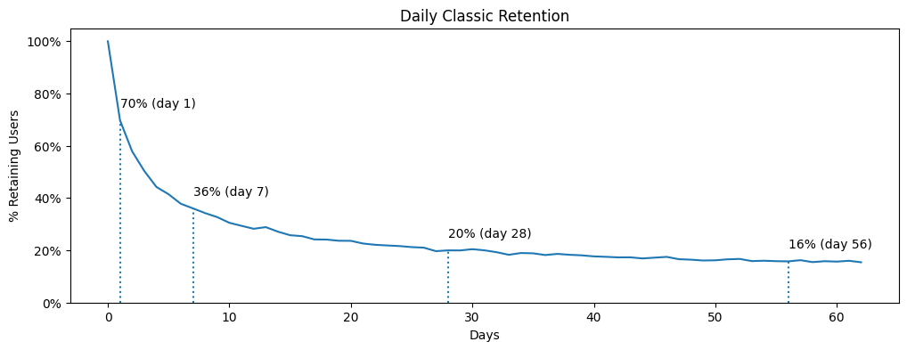
We can see that 70% of users returned the day after their first visit, 36% came back on day 7, and 20% on day 28. After roughly 30 days, the curve flattens into a plateau — a sign that the product has found Product/Market Fit.
Calculating Rolling Retention
Now let’s write a calculate_rolling_retention function. Its logic is almost identical to the previous one — with one key difference: we now select records where the day number is greater than or equal to the day we’re calculating the metric for.
Here’s that condition:
1df[df['day'] >= day]['user_id'].unique()
And here’s the full function:
 1def calculate_rolling_retention(df: pd.DataFrame, days: list) -> list:
 2
 3    # Calculate the start date for each user and merge with the original DataFrame
 4    start_date = df.groupby('user_id')['date'].min().rename("start_date")
 5    df = pd.merge(df, start_date, left_on='user_id', right_index=True)
 6
 7    # Calculate the number of days since the start date for each row
 8    df['day'] = (df['date'] - df['start_date']).dt.days
 9
10    # Create a list to store rolling retention values for each day
11    rolling_retention = []
12
13    # Calculate rolling retention for each day
14    for day in days:
15        # Select users who returned on day `day` or later
16        users_with_rolling_day = df[df['day'] >= day]['user_id'].unique()
17
18        # Calculate rolling retention for this day
19        rolling_retention.append(len(users_with_rolling_day) / len(df['user_id'].unique()))
20
21    return rolling_retention
And the results:
1days = list(range(0, 63))
2
3rolling_retention = calculate_rolling_retention(df, days)
4
5plt_show(days, rolling_retention, xs=[1, 7, 28, 56], title='Daily Rolling Retention')
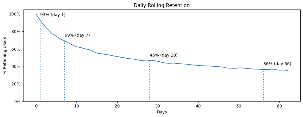
We can see that 93% of users returned to the product from day 1 onward, 69% from day 7, and 46% from day 28.
Calculating Full Retention
Finally, let’s write the function for Full Retention.
 1def calculate_full_retention(df: pd.DataFrame, days: list) -> list:
 2
 3    # Calculate the start date for each user and merge with the original DataFrame
 4    start_date = df.groupby('user_id')['date'].min().rename("start_date")
 5    df = pd.merge(df, start_date, left_on='user_id', right_index=True)
 6
 7    # Calculate the number of days since the start date for each row
 8    df['day'] = (df['date'] - df['start_date']).dt.days
 9
10    # Create a list to store full retention values for each day
11    full_retention = []
12
13    for day in days:
14        # Create the set of days we expect to see for full retention
15        expected_days = set(range(1, day + 1))
16
17        # Get unique activity days for each user
18        unique_days = df.groupby('user_id')['day'].unique()
19
20        # Identify users with full retention up to retention_day
21        full_retention_users = unique_days[unique_days.apply(lambda x: set(x) > expected_days)].index
22
23        # Calculate full retention for this day
24        full_retention.append(len(full_retention_users) / len(df['user_id'].unique()))
25
26    return full_retention
1days = list(range(0, 10))
2
3full_retention = calculate_full_retention(df, days)
4
5plt_show(days, full_retention, xs=[1, 3, 6], title='Daily Full Retention')
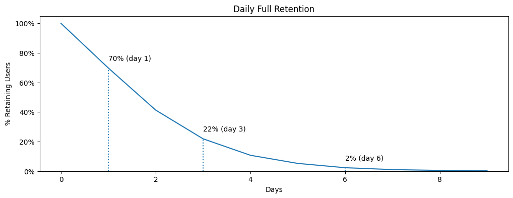
We can see that 70% of users returned to the product the day after their first visit. Since this matches the Classic Retention value, the calculations are probably correct :). 22% of users visited the product every day for 3 days straight; and only 2% visited every day for 6 consecutive days.
Takeaways
- Source code is available in [Google Colab] and on [GitHub], first of all.
- There are no universal Retention parameters that work for every product. The right metric type, window size, and benchmark values all depend on your product’s nature and current goals.
- That said, Classic Retention is more widely used than Rolling or Full Retention.
- Calculating these metrics by hand is fairly straightforward, but it takes a bit of practice with product analytics tooling.